This blog post will be Part 1 of outlining the materials and methods used in our lab’s most recent work on generating polygenic risk scores (PRSs). This article is entitled “Performance of polygenic risk scores for cancer prediction in a racially diverse academic biobank”. It was published in October 2021 and led by Dr. Louise Wang and Heena Desai.

The purpose of the study was to determine whether PRSs can improve on current risk calculators for predicting cancer occurence, particularly in non-white populations.

This blog post will not explain the entire study. Instead, I will outline the methods used. My sources for this blog post are the article, available here on Elsevier and here on PubMed, as well as a text file from Heena that explained the study process in greater detail.

Penn Medicine Biobank cohort and genotyping

Briefly, at the time of the study, there were:

• 20,079 patients
• There were 3 batches of different DNA array-based genotyping using Illumina’s “Infinium Global Screening Array (GSA)”
  • 5,676 used Illumina GSA V1 chip
  • 2,972 used Illumina GSA V2 chip at Children’s Hospital of Philadelphia (CHOP)
  • 16,940 used Illumina V2 chip at Regeneron Genetics center

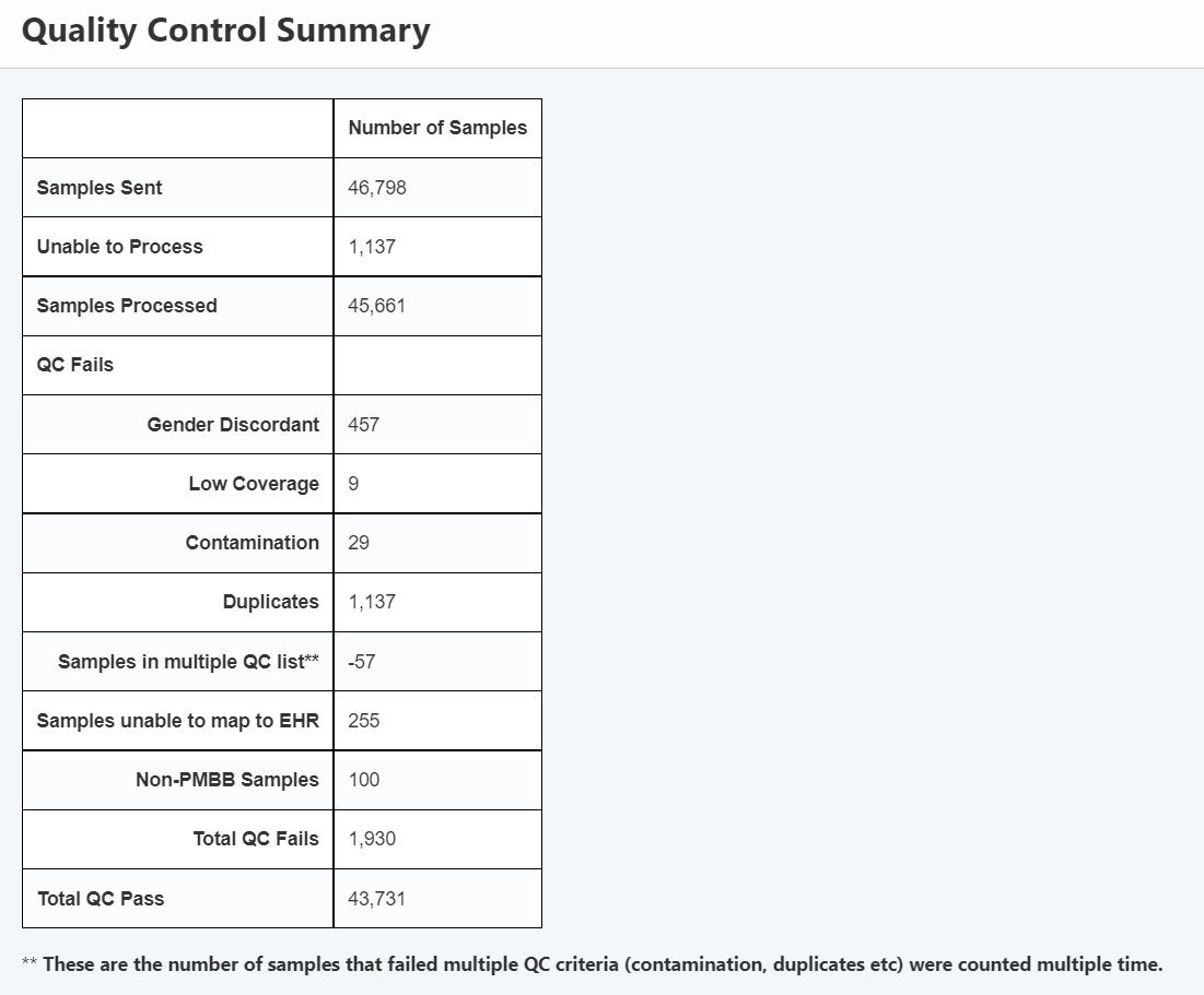
These samples had to be processed in a facility which is subject to flaws. Although this table contains newer numbers (updated after this paper), it gives a sense of how samples may not make it to final results.

Genotyping quality control and genetic ancestry determination

Genetic information used was the “exome” vcf files, which I presume were taken from the “Exome” directory and included the “pVCF” subdirectory. I believe this was the subfile called “All Variants”.

Different degrees of quality control:

It’s important to note that these exome vcf files have already undergone several steps in quality control. In fact, there are different versions of them available. They are called:

• NF which stands for non-filtered
• GL which stands for Goldilocks

Goldilocks quality control:

• For SNP variants with “depth of coverage” (DP) < 7, this is modified to “No-call”
• For INDEL variants with “depth of coverage” (DP) <10, this is modified to “No-call”
• Allele Balance (AB) filters, which detect 2 scenerios of heterozygous genotype calls, and then change a sample to “No-call”
  • SNP variant site requires at least one sample to carry an alternate Allele Balance (AB) >= 15%
  • INDEL variant sites require at least one sample to carry an alternate Allele Balance (AB) >= 20%

At this point, I believe the study used the Goldilocks file, which was converted to .bed using Plink for further processing.

Note: With this .vcf/.bed file, I wasn’t sure how each variant is linked to a patient. When I examine further, I see that the .vcf files in the Goldilocks dataset are ordered by chromosome number, and then inside the file there are PMBB id numbers. This might explain how later, we can correlate each patient phenotypic information with their genetic variants from the exome file.

• E.g for chromosome 1, there is a .vcf file called “Chromosome 1”
• Then, for the CHROM # in the .vcf file, there’s a PMBB ID, such as PMBB9408077252215

Further quality control measures:

• Sex mismatch errors
  • If the reported phenotypic sex was different than the genetic sex, the patient was removed
• Poor sample call rate
  • If genotyping had a sample call rate was <90%, patient was removed
• Palindromic variants
  • If there were palindromic variants, patient was removed
• Variants with a poor call rate
  • If the variants had a call rate <95%, patient was removed

Imputed samples:

Dislosure: I have never understood imputed samples.

Apparently, samples were imputed using Trans-Omics for Precision Medicine reference panel (TopMed) version r2.

Genetically Informed Ancestry (GIA)

The goal here was to determine whether each patient was from a European or African descent, based on genetic evaluation. I’m unclear on how this was performed. I believe this was through a combination of software or machine learning.

Through software, I believe this was through Eigensoft, of which there is an option to perform “Eigenstrat principal components analysis”. There is a script called “smartpca”. After grouping together populations using this tool, they were labelled as below.

Through machine learning, groups were labelled by taking the “1000 Genome” project samples and using them as a training set with labels. Then, PMBB samples were used as a testing set.

Given my limited understanding in these last two topics, I’ll likely need to dedicate a separate blog post on them. That’s all for today!

In Part 2 of Materials and Methods

• Phenotyping of PMBB participants
• SNV selection
• PRS generation and statistical analysis