Linkage disequilibrium - understanding the evolutionary past and mapping the medical future… A review

In this blog post, I’ll cover a paper published by Montgomery Slatkin in Nature Reviews genetics in 2008, entitled “Linkage disequilibrium - understanding the evolutionary past and mapping the medical future”. It can be found on Nature’s website here and free on Pubmed here.

During this review, I also consulted several youtube videos and blogs to provide more information about linkage disequilibrium (LD).

Background

Linkage disequilibrium is a confusing topic, yet it’s fundamental to understanding how genes are passed down and affect phenotype. This is a paper written to Montgomery Slatkin in Nature Reviews Genetics, in a series called “Fundamental Concepts in Genetics”. He describes the basic concepts of linkage disequilibrium and elaborates on how they can be used to study population genetics. Montgomery Slatkin is an American Biologist and professor at University of Berkeley.

Linkage disequilibrium and terms

Linkage disequilibrium, at its core, is the nonrandom association of alleles at different loci. Let’s unpack this

Defining terms:

• We refer to a locus as a physical location of a genes or genetic marker on the chromosome, notated by a letter e.g. “A” or “B”
• We refer to an allele as a particular version of multiple versions of a locus or gene
• For a locus with 2 alleles, we notate alleles using upper or lower case, e.g. “A” or “a”
• For a locus with more than 2 alleles, we notate using numbers, e.g. “”, “”, “”, etc.
• We notate the frequency of an allele “A” in a population with “”

Remember that for a human with 2 of each chromosome, it’s possible to have 0, 1, or 2 copies of allele “a”

For perfect Mendelian genetics, we can remind ourselves of the equation to calculate frequencies for bi-allelic genes as:

If we continue to use Mendelian gentics and we look at just one chromosome, we can calculate the frequency of particular combinations of alleles (A or a) at 2 different loci (A and B)

However, linkage disequilibrium (LD) can occur in the case that the above equations are not true. In other words, the true association of A-B, A-b, a-B, and a-b are not the same as the expected association.

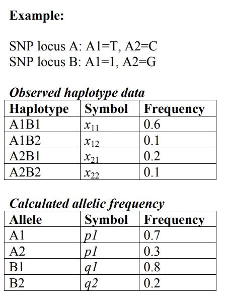
Let’s look at the example below:

In this example, the expected frequency of however the observed frequency of A1B1 is 0.6. Therefore, the loci are in some degree of linkage disequilibrium.

It’s from here that we can start to calculate the degree of LD. This is calculated using the following terms:

• D refers to the difference in observed frequency and expected frequency
• D’ refers to another value measuring the degree of linkage disequilibrium. In this case, we measure D’ from 0 (no LD) to 1 (the maximum LD that would be possible for this given pair of loci). D’ is a “scaled” version of D
• is a correlation coefficient. E.g. “to what extent do A and B go together compared to A and b?

The above statements are fairly intuitive. We can then convert them to formulas, which is far less intuitive.

Measuring LD and using it for statistics

So far, we have established that when two loci have nonrandom association, this is referred to as linkage disequilibrium. We’ve also described that this degree of LD can be measured. We can measure it in the form of D, D’, or .

In studies, these measures can’t be deemed “statistically significant”. In order to do this, we use chi squared or Fisher’s exact test.

Haplotype blocks

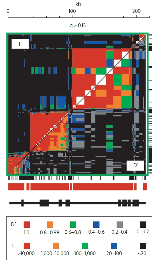
Lastly, I’d like to discuss an interesting part of the paper which describes “haplotype blocks”. To explain, this is a feature that describes how most linkage desquilibrium occurs in block-like patterns. Loci are linked to other loci in blocks from 1kb to 100kb in size. The figure below shows a segment of the major histocompatibility complex with non-overlapping sets of loci in strong LD. At the borders of these blocks, there is a “hot-spot” of recombination.

The figure shows the pattern of pairwise LD in MHC Class II in humans for all pairs of SNPs in the region for which the frequency (q) of the less common allele is >0.15. The region above the diagonal shows levels of L obtained when using D’ = O as the null hypothesis (L is the likelihood ratio from the test of linkage equilibrium).

I think this figure is so interesting! We can graphically see where recombination is happening in the genome. We can see that it isn’t random. It’s happening at specific “hot-spots” that lead to linkage disequilibrium.

The rest of the paper

The rest of the paper goes on to describe further advanced topics in linkage disequilibrium. For example, it addresses

• How to meausre linkage disequilibrium when comparing more than 2 loci
• LD between different populations
• How natural selection, genetic drift, population subdivision, population bottlenecks, inbreeding, and gene conversion impact linkage disequilibrium
• The linkage disequilibrium of gene mutations
• Impact of natural selection on LD
• Impact of allele age on LD

Take home points

Linkage disequilibrium is the non-random association of alleles at different loci. It can be quantified using measures such as D, D’, and . It can be statistically evaluated using chi-square and Fisher’s exact test. It’s a fundamental component of genetics that must be considered when evaluating the association between genes and phenotype.